Phase 3 — SVG Rendering, Cache, and the Interactive Explorer
Phase 1 inferred transitions from source code. Phase 2 extracted the full state graph into state-machines.json — 43 machines, 10 adapters, 27 edges — via the TypeScript Compiler API. Phase 3 takes that JSON and turns it into something a human can look at: an SVG diagram with every machine as a node, every edge as a routed arrow, and every node clickable to reveal its states, transitions, emits, and listens.
The rendering is not a one-shot script. It involves four distinct concerns:
- Layout — computing x/y positions for 53 nodes and 27 edges using the elkjs layered layout algorithm.
- SVG generation — converting those positions into a complete SVG fragment with styled nodes, routed polyline edges, arrow markers, and event labels.
- Caching — avoiding the expensive layout computation when the input has not changed.
- Hydration — attaching interactivity to the pre-rendered SVG in the browser: pan, zoom, selection, filtering, detail panels, and per-machine statechart popovers with an interactive simulator.
Each concern lives in its own module. The layout engine is injected via a DI seam. The cache is a pure decision function with event-driven observability. The SVG generator builds fragments from pure helpers. The explorer hydration runs in the browser and wires pure state machines to DOM effects.
This part walks through every layer, from the LayoutEngine interface to the attachSimulator function that lets users step through a machine's transitions interactively.
The LayoutEngine Interface
The renderer needs a layout engine — something that takes a list of nodes with widths and heights, a list of edges with source and target IDs, and returns computed positions for every node and routed sections for every edge. The interface is small:
export interface LayoutNodeInput {
  id:     string;
  width:  number;
  height: number;
}

export interface LayoutEdgeInput {
  id:     string;
  source: string;
  target: string;
}

export interface LayoutInput {
  nodes: LayoutNodeInput[];
  edges: LayoutEdgeInput[];
}

export interface LayoutPoint { x: number; y: number; }

export interface LayoutNodeResult {
  id:     string;
  x:      number;
  y:      number;
  width:  number;
  height: number;
}

export interface LayoutEdgeSection {
  startPoint: LayoutPoint;
  endPoint:   LayoutPoint;
  bendPoints?: LayoutPoint[];
}

export interface LayoutEdgeResult {
  id:       string;
  source:   string;
  target:   string;
  sections: LayoutEdgeSection[];
}

export interface LayoutResult {
  width:  number;
  height: number;
  nodes:  LayoutNodeResult[];
  edges:  LayoutEdgeResult[];
}

export type LayoutEngine = (input: LayoutInput) => Promise<LayoutResult>;
That is the entire contract. LayoutInput in, LayoutResult out. The engine is async because layout computation can be expensive (elkjs runs a Sugiyama-style layered algorithm with crossing minimization, and at 53 nodes it takes 50-100ms). The return type provides everything the SVG generator needs: node positions, edge polylines with bend points, and the overall canvas dimensions.
The type is a bare function signature, not a class with methods. This is deliberate. A layout engine has one job: compute positions. There is no lifecycle, no state, no configuration surface that changes between calls. A function type makes the seam as narrow as possible.
Why elkjs
The production implementation wraps the elkjs npm package — the JavaScript port of the Eclipse Layout Kernel. Three properties make it the right choice for this use case:
Layered layout. The state-machine graph is inherently layered: source machines on the left, adapters in the middle, sink machines on the right. A layered algorithm (Sugiyama) preserves this left-to-right flow naturally. Force-directed algorithms (D3-force, cola.js) would produce a tangled hairball at 53 nodes.
Orthogonal edge routing. elkjs routes edges along horizontal and vertical segments with clean right-angle bends. The result looks like a circuit diagram, not a plate of spaghetti. Each edge has a
sectionsarray withstartPoint,endPoint, and an optionalbendPointsarray — the exact data the SVG generator needs to build a polyline path.Deterministic output. Given the same input, elkjs produces the same layout every time. No random initialization, no convergence loop, no "close enough" tolerance. This means the SVG output is stable across builds — the content-hash cache can detect real changes without being fooled by floating-point drift.

The elkjs Configuration
The production makeElkLayoutEngine function wires elkjs with a specific set of layout options:
export function makeElkLayoutEngine(): LayoutEngine {
  const elk = new ELK();

  return async (input: LayoutInput): Promise<LayoutResult> => {
    const elkGraph = {
      id: 'root',
      layoutOptions: {
        'elk.algorithm':              'layered',
        'elk.direction':              'RIGHT',
        'elk.spacing.nodeNode':       '40',
        'elk.layered.spacing.nodeNodeBetweenLayers': '80',
        'elk.edgeRouting':            'ORTHOGONAL',
        'elk.layered.crossingMinimization.semiInteractive': 'true',
      },
      children: input.nodes.map(n => ({
        id: n.id, width: n.width, height: n.height,
      })),
      edges: input.edges.map(e => ({
        id: e.id, sources: [e.source], targets: [e.target],
      })),
    };

    const result = await elk.layout(elkGraph);
    // ... map result to LayoutResult
  };
}
Each option serves a specific visual purpose:
| Option | Value | Purpose |
|---|---|---|
elk.algorithm |
layered |
Sugiyama-style layered layout for directional graphs |
elk.direction |
RIGHT |
Left-to-right flow — sources on the left, sinks on the right |
elk.spacing.nodeNode |
40 |
Minimum 40px vertical gap between nodes in the same layer |
elk.layered.spacing.nodeNodeBetweenLayers |
80 |
80px horizontal gap between layers — room for edge labels |
elk.edgeRouting |
ORTHOGONAL |
Right-angle bends only — clean, readable routing |
elk.layered.crossingMinimization.semiInteractive |
true |
Respects input order when crossing counts are equal — stabilizes layout across incremental changes |
The semiInteractive crossing minimization is the key to cache stability. Without it, elkjs might reorder nodes within a layer whenever a new edge is added, which would change every node's y-position and invalidate the cache even though the graph structure barely changed. With it, the algorithm preserves the input order as a tiebreaker, so adding one edge to a 53-node graph changes only the positions of the directly affected nodes.
The Test Stub
Tests do not use elkjs. They inject a stub layout engine that returns canned coordinates:
const stubEngine: LayoutEngine = async (input): Promise<LayoutResult> => ({
  width: 100,
  height: 100,
  nodes: input.nodes.map((n, i) => ({
    id: n.id, x: i * 20, y: i * 10, width: n.width, height: n.height,
  })),
  edges: input.edges.map(e => ({
    id: e.id, source: e.source, target: e.target,
    sections: [{
      startPoint: { x: 0, y: 0 },
      endPoint:   { x: 100, y: 50 },
    }],
  })),
});
The stub places every node on a diagonal and every edge as a straight line from origin to (100, 50). This is visually meaningless — but it exercises every code path in the SVG generator. The tests verify the structure of the SVG output (correct class names, data attributes, edge paths, arrow markers) without depending on elkjs's layout algorithm. If elkjs changes its internal heuristics in a minor version bump, the unit tests still pass. Only the visual snapshot (caught by Playwright visual regression tests) would change.
This is the DI seam in practice: the pure core is testable without the expensive dependency. The thin shell wires the real dependency. The tests verify the core. The integration test verifies the shell.
renderGraphSvg — From Graph to SVG String
The entry point for SVG generation is renderGraphSvg in scripts/lib/state-machine-svg-renderer.ts:
export async function renderGraphSvg(
  graph:        StateMachineGraph,
  layoutEngine: LayoutEngine,
  options:      RendererOptions = {},
): Promise<string> {
  const opts: Required<RendererOptions> = { ...DEFAULTS, ...options };
  const layoutInput = buildLayoutInput(graph, opts);
  const layout = await layoutEngine(layoutInput);
  // ... render SVG fragments, compose into final string
}
The function does three things:
Build the layout input.
buildLayoutInputmaps the graph's machines and adapters toLayoutNodeInputentries with sizing from the options. Machine nodes are 200x64 pixels. Adapter nodes are 200x56 pixels. Edges map directly from the graph.Compute the layout. The injected engine receives the input and returns positions.
Render SVG fragments. Each node and edge becomes an SVG fragment. The fragments are composed into a complete SVG element with a viewBox, defs (arrow markers), and a transform group that applies the padding offset.
Node Rendering
Machine nodes and adapter nodes have different visual treatments:
function renderMachineNode(node: LayoutNodeResult, machine: MachineNode): string {
  const cx = node.x + node.width / 2;
  const stateCount = machine.states.length;
  const subLabel = stateCount > 0
    ? `${stateCount} state${stateCount === 1 ? '' : 's'}`
    : 'pure module';

  return `
    <g class="sm-node sm-node-machine"
       data-node-id="${escapeXml(machine.id)}"
       data-node-kind="machine"
       data-node-name="${escapeXml(machine.name)}"
       data-node-file="${escapeXml(machine.file)}"
       data-node-states="${escapeXml(machine.states.join('|'))}"
       data-node-functions="${escapeXml(machine.functions.join('|'))}"
       data-node-events="${escapeXml((machine.events ?? []).join('|'))}"
       data-node-transitions="${escapeXml(transitionsData)}"
       tabindex="0">
      <title>${escapeXml(machine.name)} ...  </title>
      <rect x="${node.x}" y="${node.y}"
            width="${node.width}" height="${node.height}"
            rx="8" ry="8" class="sm-node-bg"/>
      <text x="${cx}" y="${labelY}"
            text-anchor="middle" class="sm-node-label">
        ${escapeXml(machine.name)}
      </text>
      <text x="${cx}" y="${subLabelY}"
            text-anchor="middle" class="sm-node-sublabel">
        ${escapeXml(subLabel)}
      </text>
    </g>`;
}
Several design decisions are embedded in this fragment:
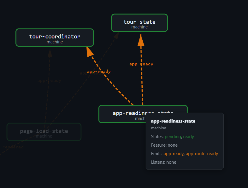
Data attributes carry machine metadata. The data-node-states, data-node-functions, data-node-events, and data-node-transitions attributes encode the machine's internal structure as pipe-delimited strings. The pipe character cannot appear in a TypeScript identifier or a state literal, so it round-trips safely. The explorer hydration reads these attributes at runtime to populate popovers and detail panels — no second JSON fetch required. The SVG itself is the data carrier.
Transitions are compact. Each transition encodes as method:from:to, joined by |. The string startLoad:idle:loading|markRendering:loading:rendering|markDone:postProcessing:done carries the full transition table for page-load-state in 90 characters. The popover parser splits on |, then on :, and has the full transition graph without a second network request.
Machine nodes are teal rounded rectangles. rx="8" ry="8" gives them a distinctive rounded-corner look. Adapter nodes use rx="4" ry="4" — slightly less rounded. The visual difference is subtle but readable: machines are the "actors" (rounded, soft), adapters are the "bridges" (sharper, utilitarian). CSS classes handle the fill colors: sm-node-machine gets a teal background, sm-node-adapter gets an orange background.
Keyboard accessible. Every node has tabindex="0" and a <title> element. Screen readers announce the machine name, state count, and file path. Keyboard users can tab through nodes and press Enter to select.
Edge Rendering
Edge rendering is more complex because of label placement:
function renderEdge(
  edge: LayoutEdgeResult,
  idx: number,
  graphEdge?: GraphEdge,
): string {
  const sectionPaths = edge.sections
    .map(s => buildPathD(edgePoints(s)))
    .join(' ');
  const isEvent = graphEdge?.kind === 'event';
  // ... build path element with appropriate class and marker
}
Three edge types exist:
| Edge Kind | Visual | Meaning |
|---|---|---|
import |
Solid arrow, current color | Module A imports module B |
event |
Dashed arrow, orange color | Module A emits an event that module B listens to |
composes |
Solid arrow, current color | Adapter A composes machine B |
Event edges get dashed strokes (stroke-dasharray="6 3") and an orange arrow marker (#sm-event-arrow). They also get a text label showing the event name, placed at the midpoint of the longest segment in the edge's polyline.
Label Placement on Edges
Label placement is the hardest visual problem in the renderer. elkjs routes edges as polylines with orthogonal segments. A naive midpoint placement — putting the label at the geometric center of the edge — stacks labels on top of each other when multiple edges converge on the same target node.
The longestSegmentMidpoint function solves this by picking the longest straight-line segment in the polyline, computing its midpoint, and offsetting the label perpendicular to the segment:
export function longestSegmentMidpoint(
  points: LayoutPoint[],
): { x: number; y: number; isHorizontal: boolean; length: number } | null {
  let bestLen = -1;
  let bestA = points[0]!;
  let bestB = points[1]!;
  for (let i = 0; i < points.length - 1; i++) {
    const a = points[i]!;
    const b = points[i + 1]!;
    const len = Math.hypot(b.x - a.x, b.y - a.y);
    if (len > bestLen) {
      bestLen = len; bestA = a; bestB = b;
    }
  }
  return {
    x: (bestA.x + bestB.x) / 2,
    y: (bestA.y + bestB.y) / 2,
    isHorizontal: Math.abs(bestB.x - bestA.x) >= Math.abs(bestB.y - bestA.y),
    length: bestLen,
  };
}
The longest segment is the widest open corridor in the edge's route — the place where a label has the most room to breathe. For horizontal segments, the label is placed above the line with a vertical offset. For vertical segments, the label is placed to the right with a horizontal offset. A small index-based jitter ((idx % 3) * 4 pixels) staggers labels when sibling edges share similar midpoints.
This heuristic is not perfect — at 27 edges, some labels still overlap. But it is far better than the naive center approach, and the interactive explorer allows zoom-in for disambiguation.
The Complete SVG
The final composition wraps everything in a root <svg> element:
return `<svg xmlns="http://www.w3.org/2000/svg"
  viewBox="0 0 ${viewW} ${viewH}"
  class="sm-explorer-svg"
  role="img"
  aria-labelledby="sm-explorer-title sm-explorer-desc">
  <title id="sm-explorer-title">State Machine Explorer</title>
  <desc id="sm-explorer-desc">
    Interactive diagram of every state machine and adapter...
    ${graph.machines.length} machines, ${graph.adapters.length} adapters,
    ${graph.edges.length} import edges.
  </desc>
  ${renderDefs()}
  <g transform="translate(${opts.padding} ${opts.padding})">
    ${edgeSvg}${nodeSvg}
  </g>
</svg>`;
The viewBox is the layout canvas plus padding on all sides. The <desc> element provides a machine-count summary for accessibility tools. Arrow markers are defined in a <defs> block and referenced by edge paths via marker-end="url(#sm-arrow)". The transform group shifts the content by the padding amount so edges touching the layout origin are not clipped.
The edges are rendered before the nodes so that node rectangles paint on top of crossing edges. This is standard SVG z-ordering: later elements paint on top of earlier ones.
RenderCache — Content-Hash Caching
The elkjs layout computation takes 50-100ms. That is fast enough for a single build, but the state-graph pipeline runs on every npm run build. If the graph has not changed — if no machine file was edited — there is no reason to re-run layout. The render cache avoids redundant work by comparing a content hash of the input graph against a persisted manifest.
The Pure Decision Logic
The cache decision is a pure function of four booleans:
export interface CacheDecisionInput {
  key:           string;
  currentHash:   string;
  manifestHash:  string | undefined;
  outputExists:  boolean;
  force?:        boolean;
}

export type CacheDecision =
  | { action: 'reuse';   reason: 'hit' }
  | { action: 'render';  reason: 'force' | 'missing-manifest' | 'hash-changed' | 'output-missing' };

export function decideCacheAction(input: CacheDecisionInput): CacheDecision {
  if (input.force)                            return { action: 'render', reason: 'force' };
  if (input.manifestHash === undefined)       return { action: 'render', reason: 'missing-manifest' };
  if (input.manifestHash !== input.currentHash) return { action: 'render', reason: 'hash-changed' };
  if (!input.outputExists)                    return { action: 'render', reason: 'output-missing' };
  return { action: 'reuse', reason: 'hit' };
}
Five input combinations, five outcomes, zero branching ambiguity. The function has no dependencies — no filesystem, no clock, no crypto. It takes strings and booleans and returns a discriminated union. Testing it is trivial:
'forces a render when force=true regardless of other state'() {
  const d = decideCacheAction({
    key: 'k', currentHash: 'a', manifestHash: 'a',
    outputExists: true, force: true,
  });
  expect(d).toEqual({ action: 'render', reason: 'force' });
}

'reuses when everything matches'() {
  const d = decideCacheAction({
    key: 'k', currentHash: 'a', manifestHash: 'a',
    outputExists: true,
  });
  expect(d).toEqual({ action: 'reuse', reason: 'hit' });
}
The decision tree reads top to bottom:

The CacheEvent Discriminated Union
Every decision and every manifest write emits a well-typed event:
export type CacheEvent =
  | { type: 'hit';                  key: string; hash: string }
  | { type: 'miss-missing-manifest'; key: string; hash: string }
  | { type: 'miss-hash-changed';    key: string; hash: string; previousHash: string }
  | { type: 'miss-output-missing';  key: string; hash: string }
  | { type: 'force';                key: string; hash: string }
  | { type: 'commit';               key: string; hash: string };
Six event types, each carrying the key and current hash, plus the miss-hash-changed variant that also carries the previous hash for diagnostic logging. The commit event fires after a successful render when the manifest is updated — it closes the loop by confirming that the new hash has been persisted.
The Emitter interface is a single-method port:
export interface Emitter {
  emit(event: CacheEvent): void;
}
Production wires a console logger that prints checkmarks and diagnostic hashes. Tests wire a recording emitter that pushes events into an array:
function makeRecorder(): Emitter & { events: CacheEvent[] } {
  const events: CacheEvent[] = [];
  return {
    events,
    emit(e) { events.push(e); },
  };
}
The event-driven approach has a concrete benefit: the CLI script does not need to format log messages itself. The emitter does it. If a future consumer needs structured logging (JSON lines, metrics, etc.), it injects a different emitter. The pure cache core never changes.
The CacheStore Interface
The manifest is a simple Record<string, string> — cache keys mapping to content hashes. The CacheStore interface abstracts read/write:
export interface CacheStore {
  read():  Record<string, string>;
  write(manifest: Record<string, string>): void;
}
Production reads from and writes to data/state-machines.svg.manifest.json. Tests use an in-memory store:
function makeInMemoryStore(
  initial: Record<string, string> = {},
): CacheStore {
  let state = { ...initial };
  return {
    read:  () => ({ ...state }),
    write: (m) => { state = { ...m }; },
  };
}
The in-memory store is synchronous. The production store wraps fs.readFileSync and fs.writeFileSync. The interface is synchronous because the cache decision itself is synchronous — the expensive async work (layout) only happens after the decision says "render." Keeping the store sync avoids an unnecessary async chain in the critical path.
canonicalGraphContent — Stable Hashing
The content hash must be stable across builds even when non-structural fields change. The generatedAt timestamp in state-machines.json changes on every extraction run. If the hash included that field, the cache would miss every time — defeating its purpose.
export function canonicalGraphContent(graph: StateMachineGraph): string {
  const { generatedAt: _ignored, ...rest } = graph;
  return JSON.stringify(rest);
}
The function strips generatedAt and serializes the rest. If only the timestamp changed, the hash stays the same and the cache hits. If a machine was added, renamed, or had its transitions modified, the hash changes and the cache misses. This is exactly the right granularity — re-render when the visual output would change, skip when it would not.
createRenderCache — Composition
The public RenderCache interface composes the hash function, the store, the decision logic, and the emitter:
export interface RenderCache {
  hash(content: string): string;
  check(input: {
    key: string; content: string;
    outputExists: boolean; force?: boolean;
  }): CacheDecision;
  commit(key: string, hash: string): void;
}

export function createRenderCache(env: RenderCacheEnv): RenderCache {
  const emit = (e: CacheEvent): void => env.emitter?.emit(e);
  return {
    hash: (content) => env.hash(content),
    check({ key, content, outputExists, force }) {
      const currentHash  = env.hash(content);
      const manifest     = env.store.read();
      const manifestHash = manifest[key];
      const decision = decideCacheAction({
        key, currentHash, manifestHash, outputExists, force,
      });
      emit(decisionEvent(decision, key, currentHash, manifestHash));
      return decision;
    },
    commit(key, hash) {
      const manifest = env.store.read();
      manifest[key] = hash;
      env.store.write(manifest);
      emit({ type: 'commit', key, hash });
    },
  };
}
The caller's workflow is:
- Call
cache.check()with the current content and output state. - If the decision is
reuse, skip rendering. - If the decision is
render, run the layout engine, write the SVG, then callcache.commit()with the new hash.
The cache never renders anything itself — it only decides. The rendering logic stays in runRender, and the cache is a consultation, not a delegation.
The render-state-machine-svg-core Module
The core module connects the SVG renderer and the cache without importing any Node-built-in modules. It depends on a FileSystem port for all I/O:
export interface RenderDeps {
  fs: FileSystem;
  root: string;
  inFile: string;       // absolute
  outFile: string;      // absolute
  manifestPath: string; // absolute
  engine: LayoutEngine;
  hash: (content: string) => string;
  cacheKey: string;
  force: boolean;
  emitter?: Emitter;
}

export type RunOutcome =
  | { action: 'reuse' }
  | { action: 'render'; sizeBytes: number; machines: number; adapters: number };
The runRender function orchestrates the full flow:
- Read
state-machines.jsonvia theFileSystemport. - Build an in-memory
CacheStoreprimed from the manifest file. - Create a
RenderCachefrom the store + hash + emitter. - Compute the canonical content and check the cache.
- If reuse, return immediately.
- If render, call
renderGraphSvgwith the layout engine, write the SVG, commit the hash, flush the manifest.
The RunOutcome union tells the caller what happened: reuse (nothing written) or render (with stats). The CLI shell uses these stats for its log line:
> data/state-machines.svg.html (42.7 KB, 43 machines, 10 adapters)In-Memory CacheStore for Pre-Read Manifests
The manifest file is read once at the start and held in memory. The makeInMemoryCacheStore function creates a CacheStore that reads and writes from a plain object:
export function makeInMemoryCacheStore(
  initial: Record<string, string>,
): CacheStore & { current: Record<string, string> } {
  const state: Record<string, string> = { ...initial };
  return {
    current: state,
    read:  () => ({ ...state }),
    write: (manifest) => {
      for (const k of Object.keys(state)) delete state[k];
      for (const [k, v] of Object.entries(manifest)) state[k] = v;
    },
  };
}
The current property exposes the live state so that runRender can flush it to disk after a commit. This avoids a second read of the manifest file — the in-memory store is always the source of truth during the render, and the disk write happens once at the end.
The Explorer UI
The SVG is pre-rendered at build time and inlined into the explorer HTML page. The browser does not re-render anything — it hydrates. The state-machines-explorer.ts module finds the pre-existing SVG, indexes its nodes and edges by their data-* attributes, and attaches interactivity through five pure state machines:
| Machine | Role | States |
|---|---|---|
svg-viewport-state |
Pan/zoom via viewBox manipulation | scale, panX, panY |
explorer-selection-state |
Hover and click tracking | hoveredId, selectedId |
explorer-filter-state |
Text + kind filtering | filterText, activeKinds |
explorer-detail-state |
Side panel open/close | open, closed |
machine-popover-state |
Per-machine modal | open, closed |
Each machine follows the same pattern as the 43 FSMs documented in Part IV: a factory function that returns a pure state machine with methods, callbacks, and no DOM access. The DOM side effects — toggling CSS classes, rendering HTML fragments, manipulating the SVG viewBox — happen in the callbacks, not in the machines.
Hydration Entry Point
The entry point is idempotent — it checks a data-sm-explorer-hydrated flag so that multiple code paths (DOMContentLoaded + SPA content swap) do not double-hydrate:
export function initStateMachinesExplorer(): void {
  const container = document.getElementById('state-machines-explorer');
  if (!container) return;
  if (container.dataset.smExplorerHydrated === '1') return;
  container.dataset.smExplorerHydrated = '1';
  void mount(container);
}
In static builds, the SVG is already in the DOM (inlined by the build-time page renderer). In dev mode, if the SVG is missing, the adapter fetches data/state-machines.svg.html via XHR and inserts it. Either way, after the SVG is present, hydrate() runs.
Node Indexing
The hydration function indexes every node and edge by their data-* attributes for O(1) lookup:
const nodeEls = svg.querySelectorAll<SVGGElement>('[data-node-id]');
const nodes = new Map<string, SVGGElement>();
const filterableNodes: FilterableNode[] = [];
nodeEls.forEach(el => {
  const id   = el.dataset.nodeId   ?? '';
  const kind = (el.dataset.nodeKind ?? 'machine') as ExplorerNodeKind;
  const name = el.dataset.nodeName  ?? id;
  nodes.set(id, el);
  filterableNodes.push({ id, kind, label: name });
});
const edges = Array.from(
  svg.querySelectorAll<SVGPathElement>('[data-edge-id]'),
);
The nodes map supports selection and detail panel lookups. The filterableNodes array supports the text-and-kind filter. The edges array supports edge highlighting when a node is selected — every edge whose data-edge-from or data-edge-to matches the selected node gets the highlighted class.
Pan/Zoom via ViewBox Manipulation
The viewport is not a CSS transform. It is an SVG viewBox attribute. The svg-viewport-state machine maintains scale, panX, panY, baseWidth, and baseHeight. The getViewBox function converts this state to a viewBox string:
viewBox = "(panX) (panY) (baseWidth / scale) (baseHeight / scale)"Zooming at 2x halves the visible area, doubling the apparent size of everything. Panning shifts the origin. The result is smooth, resolution-independent zoom that works at any display density — unlike CSS transforms, which can blur SVG content at high zoom levels.
Three interaction paths manipulate the viewport:
Wheel zoom.
container.addEventListener('wheel', ...)captures both plain wheel and ctrl+wheel.preventDefaultblocks the browser's page-zoom gesture when the cursor is over the explorer. The zoom focal point is the cursor position, converted from screen coordinates to SVG coordinates viascreenToSvg.Drag-to-pan.
pointerdownon the container (not on a node) starts a drag.pointermoveconverts pixel deltas to SVG-unit deltas and callspanBy.pointerup/pointercancelends the drag. Pointer capture ensures smooth dragging even if the cursor leaves the container.Toolbar buttons. Zoom in, zoom out, fit (reset), and fullscreen buttons call the corresponding pure functions.
Click and Selection
Clicking a node selects it. Clicking it again deselects. The selection machine toggles CSS classes on all nodes and highlights incident edges:
function applySelectionClasses(
  hoveredId: string | null,
  selectedId: string | null,
  ctx: HydrationContext,
): void {
  for (const [id, el] of ctx.nodes) {
    el.classList.toggle('hovered',  id === hoveredId);
    el.classList.toggle('selected', id === selectedId);
  }
  for (const edge of ctx.edges) {
    const from = edge.dataset.edgeFrom;
    const to   = edge.dataset.edgeTo;
    const incident = selectedId !== null
      && (from === selectedId || to === selectedId);
    edge.classList.toggle('highlighted', incident);
  }
}
Selecting a node also opens the detail panel, which shows the machine's name, file path, states, methods, and connections.
The Detail Panel
The detail panel reads metadata from the selected node's data-* attributes:
function renderDetailHtml(nodeId: string, ctx: HydrationContext): string {
  const el = ctx.nodes.get(nodeId);
  const states    = splitPipe(el.dataset.nodeStates);
  const functions = splitPipe(el.dataset.nodeFunctions);

  const neighbours: { id: string; direction: 'in' | 'out' }[] = [];
  for (const edge of ctx.edges) {
    if (edge.dataset.edgeFrom === nodeId)
      neighbours.push({ id: edge.dataset.edgeTo!, direction: 'out' });
    if (edge.dataset.edgeTo === nodeId)
      neighbours.push({ id: edge.dataset.edgeFrom!, direction: 'in' });
  }
  // ... render HTML with states, methods, connections
}
The splitPipe utility splits a pipe-delimited string back into an array — the inverse of the join('|') used during SVG generation. No second data source is consulted. The SVG is self-describing.
The Popover — Per-Machine Statechart
Double-clicking a machine node opens a modal popover showing that machine's internal state diagram. The popover reads the data-node-transitions attribute, parses it into a transition array, and passes it to renderMachineStateDiagram — a pure function that produces an SVG statechart with state bubbles and transition arrows:
const transitions = (el.dataset.nodeTransitions ?? '')
  .split('|').filter(Boolean)
  .map(entry => {
    const [method = '', from = '*', to = ''] = entry.split(':');
    return { method, from, to };
  });

const diagram = renderMachineStateDiagram(
  { name, states, methods: functions, transitions, events },
  { ariaLabel: `State diagram for ${name}` },
);
The statechart is interactive: it has its own pan/zoom via attachDiagramZoom, and it hosts an FSM simulator.
The FSM Simulator
The simulator lets users step through a machine's transitions interactively. It shows the current state, a list of available events (methods that can fire from the current state), and a history of fired transitions:
const sim = createFsmSimulator({
  onStateChange: (current, available, history) => {
    // 1) Toggle active-state class on state bubbles
    stateEls.forEach((el, name) => {
      el.classList.toggle('msd-state--active', name === current);
    });
    // 2) Mark transition arcs available/unavailable
    for (const el of transEls) {
      const method = el.dataset.transMethod ?? '';
      const from   = el.dataset.transFrom   ?? '';
      const isAvail = available.includes(method)
        && (from === current || from === '*');
      el.classList.toggle('msd-transition-group--available', isAvail);
    }
    // 3) Rebuild event buttons
    // 4) Rebuild history list
  },
});

sim.init(transitions, initialState);
The pickInitialState heuristic selects the starting state: it prefers common initial-state names (idle, initial, closed, start), falls back to a state with outgoing transitions, and as a last resort uses the first state in the union. The user can fire events by clicking buttons, and the simulator highlights the active state in the statechart SVG, dims unavailable transitions, and records each fired event in the history list.
A "Reset" button returns the machine to its initial state. If the machine reaches a terminal state (no outgoing transitions), the buttons area shows "(terminal -- reset to replay)".
Filtering
The explorer supports two filter dimensions:
Text filter. A text input matches against node labels. Typing "page" shows only nodes whose name contains "page" (case-insensitive).
Kind filter. Checkboxes for "machine" and "adapter" toggle which node types are visible.
The explorer-filter-state machine tracks the filter text and the set of active kinds. The applyFilter function iterates over all nodes, checks filter.matches(node), and toggles the filtered-out class. Edges are hidden when both endpoints are filtered out.
Global Event Handling
The explorer handles three global events:
- Escape key. Closes the popover (if open), or dismisses the detail panel.
- Outside click. Clicking outside the detail panel (and not on a node or the container) dismisses it.
- Fullscreen change. Updates the fullscreen button text and closes the popover when the user exits fullscreen via Escape.
These handlers use the pure shouldCloseOnKeydown and shouldCloseOnDocumentClick functions from the panel-events module — the same functions that drive the detail panels elsewhere in the application.
The Full Pipeline
The complete build:state-graph pipeline runs four scripts in sequence:
npm run build:state-graphWhich expands to:
npx tsx scripts/infer-fsm-transitions.ts --patch \
  && npx tsx scripts/extract-state-machines.ts \
  && npx tsx scripts/render-state-machine-svg.ts \
  && npx tsx scripts/render-fsm-composition.ts
Each step feeds the next:

| Step | Script | Input | Output | Duration |
|---|---|---|---|---|
| 1 | infer-fsm-transitions.ts --patch |
src/lib/*.ts |
patched src/lib/*.ts |
~200ms |
| 2 | extract-state-machines.ts |
src/lib/*.ts |
data/state-machines.json |
~300ms |
| 3a | render-state-machine-svg.ts |
data/state-machines.json |
data/state-machines.svg.html |
~100ms (cache hit) or ~600ms (miss) |
| 3b | render-fsm-composition.ts |
data/state-machines.json |
data/fsm-composition.json |
~50ms |
The total pipeline takes under 700ms on a cache hit and under 1.2 seconds on a miss. The cache saves the 500ms elkjs layout computation — significant on repeated builds during development.
Incremental Behavior
The cache makes the pipeline semi-incremental:
Phase 1 always runs but is cheap (~200ms). It only patches files that lack transitions, and after the first run all 43 machines have explicit transitions, so subsequent runs are no-ops that just verify the transitions are present.
Phase 2 always runs (~300ms). It could be cached similarly, but the extraction is fast enough that the complexity is not justified.
Phase 3a checks the cache before layout. If the input graph has not changed (same machines, same edges, same metadata), the cache hits and the script exits in under 100ms.
Phase 3b always runs (~50ms). The composition graph is a simple transform with no expensive computation.
The key insight: the expensive operation is layout, and layout is the one operation that is cached. Everything else is fast enough to run unconditionally.
Step 1 Output: Patched Decorators
Phase 1 reads every machine file, infers transitions where missing, and writes the inferred transitions back into the @FiniteStateMachine decorator. After the first run, every decorator has an explicit transitions array. Subsequent runs verify the array is present and report any machines that have regressed.
Step 2 Output: state-machines.json
Phase 2 walks every source file with the TypeScript Compiler API, extracts every @FiniteStateMachine decorator, and builds the StateMachineGraph:
{
  "generatedAt": "2026-04-12T10:30:00.000Z",
  "machines": [
    {
      "id": "machine:page-load-state",
      "name": "page-load-state",
      "file": "src/lib/page-load-state.ts",
      "states": ["idle", "loading", "rendering", "postProcessing", "done", "error"],
      "transitions": [
        { "method": "startLoad", "from": "idle", "to": "loading" },
        { "method": "markRendering", "from": "loading", "to": "rendering" }
      ],
      "emits": ["app-ready", "toc-headings-rendered"],
      "listens": [],
      "feature": { "id": "PAGE-LOAD", "ac": "fullLifecycle" }
    }
  ],
  "adapters": [...],
  "edges": [...]
}
Step 3a Output: state-machines.svg.html
Phase 3a produces a complete SVG fragment — no HTML wrapper, no <html> or <body>, just the <svg> element with all nodes, edges, markers, and accessibility annotations. This fragment is inlined into the explorer page by the build-time page renderer via the include: frontmatter mechanism. The file is typically 40-45 KB.
Step 3b Output: fsm-composition.json
Phase 3b produces a D3-ready graph of FSM composition, event coupling, and adapter wiring. This JSON is consumed by the composition visualizer — a separate page that shows how machines relate to each other through events and adapters. The structure follows the D3 force-graph convention: a nodes array and a links array.
The CLI Shells
Each script in the pipeline is a thin CLI shell that wires the real filesystem, the real crypto module, and the real elkjs engine to the pure core:
// render-state-machine-svg.ts — the CLI shell

import { promises as fsp } from 'fs';
import * as path from 'path';
import { createHash } from 'crypto';
import ELK from 'elkjs/lib/elk.bundled.js';
import { runRender, makeConsoleEmitter } from './lib/render-state-machine-svg-core';

const realFileSystem: FileSystem = {
  async readFile(p, enc) { return fsp.readFile(p, enc); },
  async writeFile(p, c) { await fsp.writeFile(p, c, 'utf8'); },
  async exists(p) {
    try { await fsp.access(p); return true; } catch { return false; }
  },
  async mkdir(p, opts) { await fsp.mkdir(p, opts); },
  async readdir(p) { return fsp.readdir(p); },
  async stat(p) {
    const st = await fsp.stat(p);
    return { mtimeMs: st.mtimeMs, size: st.size, isDirectory: () => st.isDirectory() };
  },
};

function sha256Hex(content: string): string {
  return createHash('sha256').update(content).digest('hex').slice(0, 16);
}

async function main(): Promise<void> {
  const force = process.argv.includes('--force');
  const outcome = await runRender(
    {
      fs: realFileSystem,
      root: ROOT,
      inFile: IN_FILE,
      outFile: OUT_FILE,
      manifestPath: MANIFEST_FILE,
      engine: makeElkLayoutEngine(),
      hash: sha256Hex,
      cacheKey: CACHE_KEY,
      force,
      emitter: makeConsoleEmitter((msg) => console.log(msg)),
    },
    path.dirname,
  );
  // ... log outcome
}
The shell is 134 lines. It imports fs, path, crypto, and elkjs — the four things the pure core does not touch. The pure core (render-state-machine-svg-core.ts) is 163 lines and imports only type interfaces. The SVG renderer (state-machine-svg-renderer.ts) is 316 lines and imports only the extractor types.
The boundary is clear:
| Module | Lines | Imports | Side Effects | Testable With |
|---|---|---|---|---|
state-machine-svg-renderer.ts |
316 | types only | none | stub layout engine |
render-cache.ts |
135 | none | none | in-memory store + recorder |
render-state-machine-svg-core.ts |
163 | types only | none | memory filesystem + stub engine |
render-state-machine-svg.ts (shell) |
134 | fs, crypto, elkjs | filesystem, process | integration test only |
The pure core is 614 lines, fully unit-tested at 100% coverage. The shell is 134 lines, tested only by the integration test that runs the full pipeline. This ratio — 82% pure, 18% shell — is the result of a deliberate architecture: push every decision into the pure core, leave only wiring in the shell.
The Contrast
The shell does four things:
- Constructs the
FileSystemadapter from Node'sfs.promises. - Constructs the
LayoutEngineadapter fromelkjs. - Constructs the hash function from
crypto.createHash. - Passes them to
runRenderand logs the result.
It does not make decisions. It does not format SVG. It does not check the cache. It does not compute hashes. Those are all pure operations that live in testable modules. The shell is glue code — and glue code is the one thing you do not unit-test, because it has no logic to verify. You test it by running the whole pipeline and checking the output, which is what the Playwright E2E tests do.
Putting It All Together
The state-machine explorer is the visible output of a four-layer architecture:
Metadata layer —
@FiniteStateMachinedecorators on 43 companion classes, carrying states, transitions, emits, listens, guards, and feature links.Extraction layer — TypeScript Compiler API walking every source file, building
StateMachineGraphwith typedMachineNode,AdapterNode, andGraphEdgeentries.Rendering layer — elkjs layout, SVG fragment builders, content-hash cache, and the thin CLI shell that wires them.
Hydration layer — five pure state machines (viewport, selection, filter, detail, popover) attached to the pre-rendered SVG in the browser, providing pan/zoom, click-to-select, text filtering, detail panels, per-machine statechart popovers, and an interactive FSM simulator.
Every layer is testable in isolation. The extraction layer's tests pass in-memory TypeScript source files. The rendering layer's tests pass a stub layout engine and a memory filesystem. The hydration layer's machines are tested as pure state machines with no DOM. The only layer that requires a real browser is the Playwright E2E test that verifies the integrated experience — and even that test runs against the static build, not a dev server.
The cache makes the pipeline incremental. The DI seams make it testable. The data-attribute encoding makes the SVG self-describing. The pure machines make the UI predictable. Each decision reinforces the others, and the result is a build-time tool that produces an interactive architectural diagram — from source code to clickable, zoomable, simulatable SVG — in under two seconds.
Continue to Part XI: Feature Traceability and the Quality Gate Chain →